Loss 函数

这次仍然是在 CIFAR-10 这一数据集上进行处理。

第一个任务是实现linear_svm.py 中 Loss 函数求导的部分，要求用朴素方法实现（带循环的）。完成后的svm_loss_naive如下：

def svm_loss_naive(W, X, y, reg):
    """
    Structured SVM loss function, naive implementation (with loops).

    Inputs have dimension D, there are C classes, and we operate on minibatches
    of N examples.

    Inputs:
    - W: A numpy array of shape (D, C) containing weights.
    - X: A numpy array of shape (N, D) containing a minibatch of data.
    - y: A numpy array of shape (N,) containing training labels; y[i] = c means
      that X[i] has label c, where 0 <= c < C.
    - reg: (float) regularization strength

    Returns a tuple of:
    - loss as single float
    - gradient with respect to weights W; an array of same shape as W
    """
    dW = np.zeros(W.shape)  # initialize the gradient as zero

    # compute the loss and the gradient
    num_classes = W.shape[1]
    num_train = X.shape[0]
    loss = 0.0
    for i in range(num_train):
        scores = X[i].dot(W)
        correct_class_score = scores[y[i]]
        for j in range(num_classes):
            if j == y[i]:
                continue
            margin = scores[j] - correct_class_score + 1  # note delta = 1
            if margin > 0:
                loss += margin
                dW[:,j] += X[i].T
                dW[:,y[i]] -= X[i].T

    # Right now the loss is a sum over all training examples, but we want it
    # to be an average instead so we divide by num_train.
    loss /= num_train

    # Add regularization to the loss.
    loss += reg * np.sum(W * W)

    #############################################################################
    # TODO:                                                                  #
    # Compute the gradient of the loss function and store it dW.                #
    # Rather that first computing the loss and then computing the derivative,   #
    # it may be simpler to compute the derivative at the same time that the  #
    # loss is being computed. As a result you may need to modify some of the    #
    # code above to compute the gradient.                                      #
    #############################################################################
    # *****START OF YOUR CODE (DO NOT DELETE/MODIFY THIS LINE)*****

    dW /= num_train
    dW += reg * 2 * W

    # *****END OF YOUR CODE (DO NOT DELETE/MODIFY THIS LINE)*****

    return loss, dW

通过数值解对解析解进行检验，检验结果如下图所示：

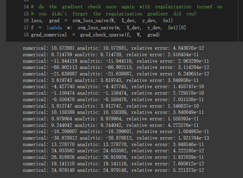
误差均在可接受范围之内。

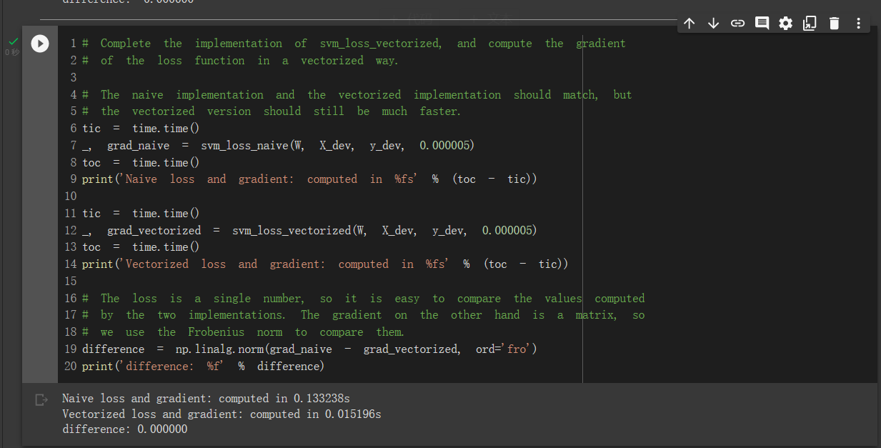
紧接着自然是向量化写法。完成后的svm_loss_vectorized如下：

def svm_loss_vectorized(W, X, y, reg):
    """
    Structured SVM loss function, vectorized implementation.

    Inputs and outputs are the same as svm_loss_naive.
    """
    loss = 0.0
    dW = np.zeros(W.shape)  # initialize the gradient as zero

    #############################################################################
    # TODO:                                                                  #
    # Implement a vectorized version of the structured SVM loss, storing the    #
    # result in loss.                                                          #
    #############################################################################
    # *****START OF YOUR CODE (DO NOT DELETE/MODIFY THIS LINE)*****

    num_classes = W.shape[1]
    num_train = X.shape[0]

    score = X.dot(W).T
    choose = np.choose(y, score)
    score =  score-choose+1
    score = np.maximum(score, 0)
    margin = score.T
    margin[np.arange(num_train),y] = 0

    loss += np.sum(margin)
    loss /= num_train
    loss += reg * np.sum(W * W)

    # *****END OF YOUR CODE (DO NOT DELETE/MODIFY THIS LINE)*****

    #############################################################################
    # TODO:                                                                  #
    # Implement a vectorized version of the gradient for the structured SVM  #
    # loss, storing the result in dW.                                          #
    #                                                                          #
    # Hint: Instead of computing the gradient from scratch, it may be easier    #
    # to reuse some of the intermediate values that you used to compute the  #
    # loss.                                                                  #
    #############################################################################
    # *****START OF YOUR CODE (DO NOT DELETE/MODIFY THIS LINE)*****

    k = np.zeros(margin.shape)
    k[margin>0] = 1
    row = np.sum(k, 1)
    k[np.arange(num_train), y] -= row.T

    dW = X.T.dot(k)
    dW /= num_train
    dW += reg * 2 * W

    # *****END OF YOUR CODE (DO NOT DELETE/MODIFY THIS LINE)*****

    return loss, dW

数值检验结果如下图所示：

梯度下降

完成了 Loss 函数之后，就要进入训练过程了。首先补全linear_classifier.py中的LinearClassifier.train()。这一函数的作用是，每一个 iteration 中选出 batch_size 个训练样本投入到 SVM 中，然后再计算一次 Loss 函数进行梯度下降，避免计算太频繁导致时间消耗过大。

完善后的LinearClassifier.train()如下：

    def train(
        self,
        X,
        y,
        learning_rate=1e-3,
        reg=1e-5,
        num_iters=100,
        batch_size=200,
        verbose=False,
    ):
        """
        Train this linear classifier using stochastic gradient descent.

        Inputs:
        - X: A numpy array of shape (N, D) containing training data; there are N
          training samples each of dimension D.
        - y: A numpy array of shape (N,) containing training labels; y[i] = c
          means that X[i] has label 0 <= c < C for C classes.
        - learning_rate: (float) learning rate for optimization.
        - reg: (float) regularization strength.
        - num_iters: (integer) number of steps to take when optimizing
        - batch_size: (integer) number of training examples to use at each step.
        - verbose: (boolean) If true, print progress during optimization.

        Outputs:
        A list containing the value of the loss function at each training iteration.
        """
        num_train, dim = X.shape
        num_classes = (
            np.max(y) + 1
        )  # assume y takes values 0...K-1 where K is number of classes

        if self.W is None:
            # lazily initialize W
            self.W = 0.001 * np.random.randn(dim, num_classes)

        # Run stochastic gradient descent to optimize W
        loss_history = []
        for it in range(num_iters):
            X_batch = None
            y_batch = None

            #########################################################################
            # TODO:                                                              #
            # Sample batch_size elements from the training data and their          #
            # corresponding labels to use in this round of gradient descent.        #
            # Store the data in X_batch and their corresponding labels in          #
            # y_batch; after sampling X_batch should have shape (batch_size, dim)   #
            # and y_batch should have shape (batch_size,)                          #
            #                                                                      #
            # Hint: Use np.random.choice to generate indices. Sampling with      #
            # replacement is faster than sampling without replacement.            #
            #########################################################################
            # *****START OF YOUR CODE (DO NOT DELETE/MODIFY THIS LINE)*****

            choice = np.random.choice(a=num_train, size=batch_size, replace=False, p=None)
            X_batch = X[choice]
            y_batch = y[choice]

            # *****END OF YOUR CODE (DO NOT DELETE/MODIFY THIS LINE)*****

            # evaluate loss and gradient
            loss, grad = self.loss(X_batch, y_batch, reg)
            loss_history.append(loss)

            # perform parameter update
            #########################################################################
            # TODO:                                                              #
            # Update the weights using the gradient and the learning rate.        #
            #########################################################################
            # *****START OF YOUR CODE (DO NOT DELETE/MODIFY THIS LINE)*****

            self.W -= learning_rate * grad

            # *****END OF YOUR CODE (DO NOT DELETE/MODIFY THIS LINE)*****

            if verbose and it % 100 == 0:
                print("iteration %d / %d: loss %f" % (it, num_iters, loss))

        return loss_history

有两部分需要补全，第一个是随机选择数据，第二个是梯度下降，实现都比较简单。

之后的训练效果：

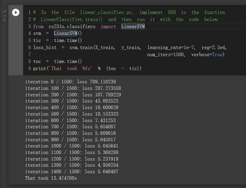
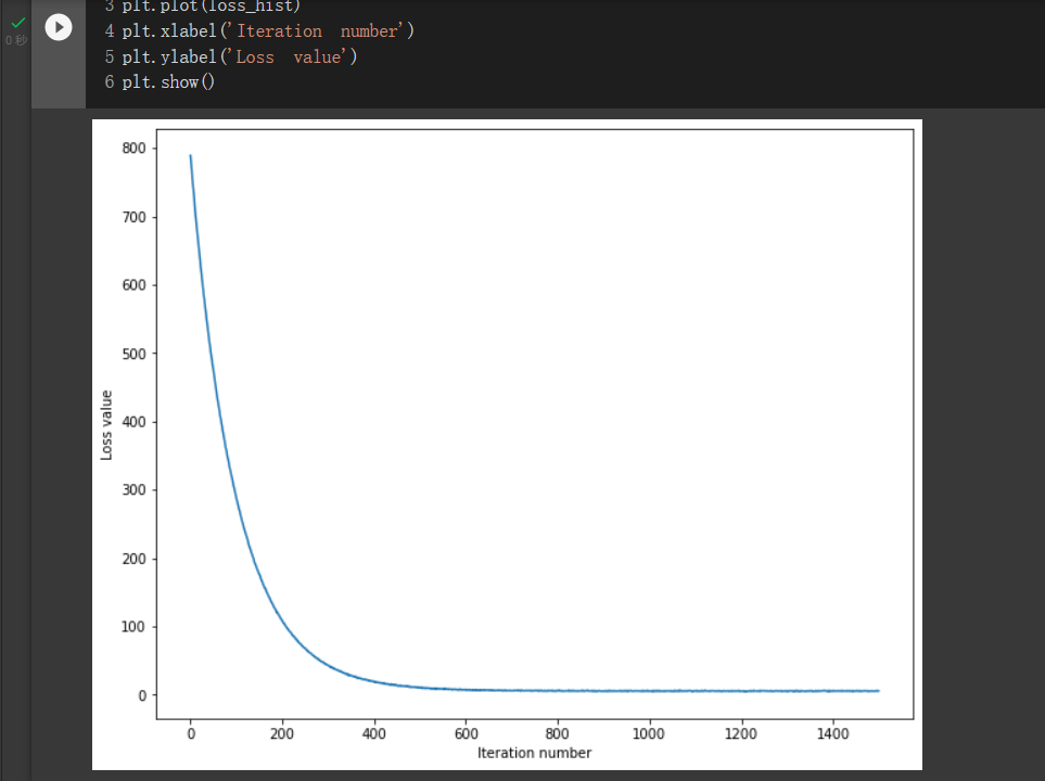
可以看出 Loss 下降还是非常明显的，代码实现没有问题。

继续完善LinearSVM.predict()，得到训练集与验证集上的准确率：

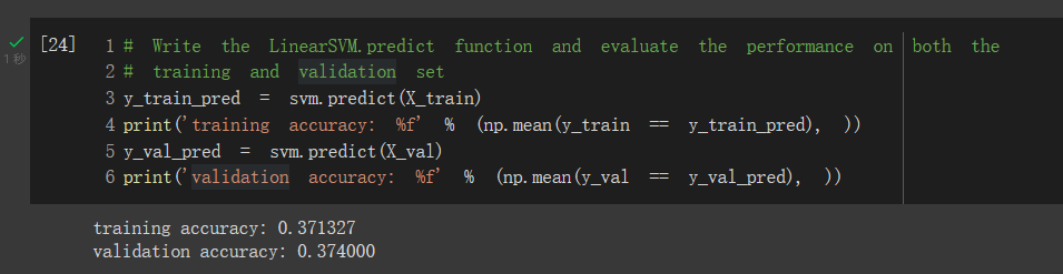
后面是调参环节，从不同的 learning rate 与 regularization strengths 中选出使验证集正确率最高的组合。对每一种组合都训一遍 SVM，然后计算一次正确率。不过在 learning rate 较大的两个情况训练时，发生了计算溢出的情况。题面中说这是正常现象，正确率接近39\%​就算成功。我本地训练最好的结果是39.6\%​，随后参考了一下别人的代码，写法上一模一样，但是人家就能达到40\%​​的正确率。。。只能说脸比较黑，初始位置选取不是太好。

补全后的调参代码如下：

# Use the validation set to tune hyperparameters (regularization strength and
# learning rate). You should experiment with different ranges for the learning
# rates and regularization strengths; if you are careful you should be able to
# get a classification accuracy of about 0.39 on the validation set.

# Note: you may see runtime/overflow warnings during hyper-parameter search. 
# This may be caused by extreme values, and is not a bug.

# results is dictionary mapping tuples of the form
# (learning_rate, regularization_strength) to tuples of the form
# (training_accuracy, validation_accuracy). The accuracy is simply the fraction
# of data points that are correctly classified.
results = {}
best_val = -1   # The highest validation accuracy that we have seen so far.
best_svm = None # The LinearSVM object that achieved the highest validation rate.

################################################################################
# TODO:                                                                        #
# Write code that chooses the best hyperparameters by tuning on the validation #
# set. For each combination of hyperparameters, train a linear SVM on the      #
# training set, compute its accuracy on the training and validation sets, and  #
# store these numbers in the results dictionary. In addition, store the best   #
# validation accuracy in best_val and the LinearSVM object that achieves this  #
# accuracy in best_svm.                                                        #
#                                                                              #
# Hint: You should use a small value for num_iters as you develop your         #
# validation code so that the SVMs don't take much time to train; once you are #
# confident that your validation code works, you should rerun the validation   #
# code with a larger value for num_iters.                                      #
################################################################################

# Provided as a reference. You may or may not want to change these hyperparameters
learning_rates = [1e-7, 5e-6]
regularization_strengths = [2.5e4, 5e4]

# *****START OF YOUR CODE (DO NOT DELETE/MODIFY THIS LINE)*****

for lr in learning_rates:
    for reg in regularization_strengths:
        svm = LinearSVM()
        svm.train(X_train, y_train, learning_rate=lr, reg=reg, num_iters=1500, verbose=True)
        y_train_pred = np.mean(y_train == svm.predict(X_train))
        y_val_pred = np.mean(y_val == svm.predict(X_val))
        results[(lr, reg)] = (y_train_pred, y_val_pred)
        if y_val_pred > best_val:
            best_val = y_val_pred
            best_svm = svm

# *****END OF YOUR CODE (DO NOT DELETE/MODIFY THIS LINE)*****

# Print out results.
for lr, reg in sorted(results):
    train_accuracy, val_accuracy = results[(lr, reg)]
    print('lr %e reg %e train accuracy: %f val accuracy: %f' % (
                lr, reg, train_accuracy, val_accuracy))

print('best validation accuracy achieved during cross-validation: %f' % best_val)

最终在测试集上取得了37.3\%的效果，将权重可视化之后，发现学习到的分类器如下图所示：

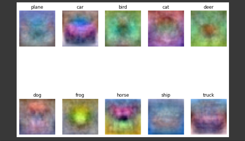
效果挺有趣，能看出学了一个轮廓以及颜色出来。

Inline Question

Q1

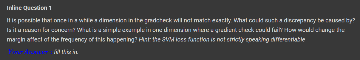
梯度不完全匹配的原因可能有浮点误差，以及数值解与解析解之间的精度误差，解析解本身也可能会和实际梯度有所偏差。这是因为所要求导的函数在原点处是不可微的，所以如果求导的位置与原点过于接近的话，解析解就可能出现误差。

这些情况对实际求解并没有太大影响。想要追求更高的验证精度可以减小\Delta x。

Q2

第i​​层权重像第i​​个分类所对应的物体的图片。这是因为 SVM 会通过二者的相似程度来进行打分，所以为了使某一种类的分数比其他种类高，SVM 就会尽可能记住这个种类比较普遍的特点。所以将权重可视化之后会像对应分类的物体。

感想

这一次对 numpy 的熟练度要求更高了，且更具有技巧性。向量法求 Loss 函数那里卡了很久，一直没有想好怎么把朴素解法的 if 给去掉。参考了别人的答案后才发现可以借助另一个矩阵进行求解。后面的实现相对来说比较简单，一路做下去没有太大压力。

目前的内容还没有涉及较为复杂的数学推导，理解起来也很轻松（可能和我之前有一定基础有关）。马上就要到神经网络部分了，希望在完成后面的习题的时候可以多多尝试一些在这块学到的 numpy 技巧，刷网课的速度也要加快了，时间不多了。